MAJIQ-SPEL
Sampling Primers for Evaluating LSVs
Background
Splicing is the process by which the spliceosome removes introns from a pre-mRNA and ligates together exons to make the final mRNA transcript. Over 95% of multi-exon genes in humans undergo some form of alternative splicing (AS), where different segments of the pre-mRNA are either removed or retained in the final mRNA. This creates different isoforms from the same pre-mRNA transcript which expands proteome diversity by encoding different versions of the same protein, and/or can alter several aspects of the mRNA’s downstream processing (e.g. localization, stability, translational efficiency, etc.). AS is tightly regulated between tissues, across development, and is often dysregulated in disease, meaning an accurate definition and quantification from RNA-sequencing data (RNA-Seq) is key for downstream analysis.
MAJIQ defines and quantifies alternative splicing through Local Splicing Variations (LSVs). LSVs are defined as multiple edges in a splice graph where several edges either come into or from a single exon. This is done through a two step process with MAJIQ. First, the Builder uses a transcriptome annotation file (gff3) that is supplemented with the user’s RNA-Seq data to construct Local Splicing Variations. Second, the Quantifier estimates the relative inclusion level for each junction in the LSV either within a single condition (PSI) or between two conditions (delta PSI). Finally, Voila is used to visualize MAJIQ’s splice graph and LSV data.
Together MAJIQ and Voila let users define, quantify, and visualize splicing variations in a robust, accurate way and compares favorably to other splicing quantification algorithms. Importantly, the LSV formulation not only captures classical alternative splicing events (e.g. cassette exons, alternative splice sites, etc.), but also allows for definition and quantification of non-classical and complex splicing variations (i.e. those involving more than three junctions). Additionally, MAJIQ allows for de novo detection of splice junctions not in the annotation database.
Around 30% of the LSVs in a given RNA-Seq experiment will involve complex LSVs, which can involve multiple exons and/or alternative splice sites. In such cases, the the number of putative isoforms that can be produced quickly becomes difficult to visualize and interpret in downstream analysis. Furthermore, no currently available tool allows users to design primers for RT-PCR, the gold standard in the field, for experimental validation of either classical or complex alternative splicing patterns.
For these reasons, we developed MAJIQ-SPEL (MAJIQ for Sampling Primers and Evaluating LSVs) which aids in the visualization, interpretation, and experimental validation of both classical and complex splicing variations.
Overview
MAJIQ-SPEL was created to assist users in several tasks related to interpretation and downstream analysis of MAJIQ’s LSVs:
- Visualizing and quantifying local isoform variations created by an LSV
- The design of RT-PCR primers for experimental validation
- Downstream functional analysis of splicing variations through connections to UCSC Genome Browser
1. Visualizing local isoform variations
LSVs involve two or more junctions that either emanate out from a reference exon (source LSV) or converge into a reference exon (target LSV). LSVs often involve multiple exons and/or alternative splice sites, some of which are connected via splice junctions not directly quantified by the LSV (see dashed lines in splice graphs for a target LSV below). These combinations can quickly become complex and thus difficult to interpret for users. To make interpretation of possible local isoform variations created from an LSV easy, MAJIQ-SPEL traverses all possible paths in the splice graph to generate an isoform table that lists the local isoform variations created by the LSV of interest.
2. Design of RT-PCR primers
MAJIQ-SPEL produces a table of putative forward and reverse primers for the 5’ most and 3’ most exons within an LSV in order to streamline primer design for users. These primers are optimized for a low-cycle RT-PCR assay, but users can adjust various parameters using advanced options. By clicking a forward and reverse primer pair, the isoform table will calculate all of the expected product sizes for the various local isoforms making primer design for both classical and complex splicing patterns quick and easy.
3. Downstream functional analysis
MAJIQ-SPEL connects to UCSC Genome Browser to upload a number of custom tracks that facilitate downstream, functional analysis. This includes coordinate information for all junctions, exons, possible intron retentions, forward, and reverse primers. Importantly, this also includes Pfam annotated protein domain track, which can aid users in exploring the possible functional consequences of these local isoform variations to resultant proteins. Users can supplement this output with their own custom tracks (e.g. RNA-Seq reads, CLIP-Seq peaks for an RBP of interest, etc.).
Walk Through
To design a primer with MAJIQ-SPEL, the MAJIQ pipeline (version 1.0.0) will have to be completed. This includes running the Builder, Quantifier, and Voila’s visualization. To run the Builder, we’ll run the following command.
majiq build ensembl.mm10.gff3 --conf config.txt --output majiq_build
The ensembl.mm10.gff3 file can be found on the MAJIQ home page and the configuration file is the following. Here we are comparing two experimental groups (adrenal gland (Adr) and cerebellum (Cer)) which each consist of three replicates.
[info]
            readlen=101
            samdir=”Location of BAM files”
            genome= mm10
            genome_path=”Location of genomic data”
            [experiments]
            Adr=Adr_CT22.mm10.sorted,Adr_CT28.mm10.sorted,Adr_CT34.mm10.sorted
            Cer=Cer_CT22.mm10.sorted,Cer_CT28.mm10.sorted,Cer_CT34.mm10.sorted
Once the Builder has completed, we can use the following command to run the Quantifier. Here we run deltapsi to compare splicing changes between the two experimental groups.
majiq deltapsi -grp1 majiq_build/Cer_CT*.mm10.sorted.majiq.hdf5 -grp2 majiq_build/Adr_CT*.mm10.sorted.majiq.hdf5 --output majiq_deltapsi_Cer_Adr --name Cer Adr
To run Voila we’ll need both the voila file and the splice graph file. The Voila file is located in the Cer_Adr directory from the Majiq delta-psi run and the splice graph file is in the output directory from the Builder’s run. We can use the following command to run Voila.
voila deltapsi Cer_Adr/Cer_Adr.deltapsi.voila --splice-graph output/splicegraph.hdf5 --output voila_deltapsi_Cer_Adr --lsv-ids-file example_LSV_list
For this example, we didn’t want an output of all the found LSVs. So, the argument “--lsv-ids-file” was included to search for just five of the LSVs. The file “example_LSV_list” is a newline separated list of the LSV IDs we wanted to remain in the visualization output.
For additional information regarding MAJIQ, Voila, and LSVs please see (Vaquero-Garcia, et al. 2016, majiq.biociphers.org).
Now that the Voila run is complete, we can now show how we get LSV data into MAJIQ-SPEL. This includes selecting a LSV, copying the required data, and pasting it into the MAJIQ-SPEL galaxy tool. Let’s start by viewing the visualization for the above voila run: http://majiq.biociphers.org/green_et_al_2017/examples.
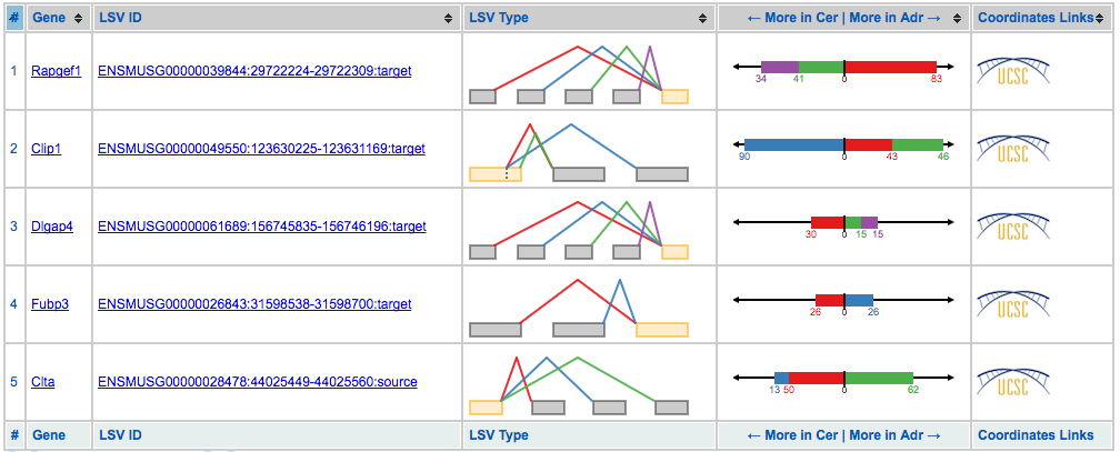
Once at this page, click a LSV ID or gene name, this brings us to the summary page for the gene that contains the selected LSV.
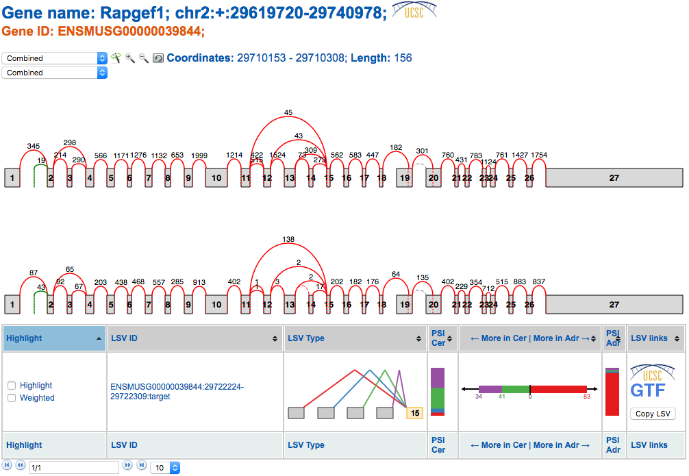
At the top we see the splice graphs for the gene and the reads for each junction for the two experimental conditions, cerebellum (top) and adrenal (bottom). In the table beneath the splice graph is the LSV for this gene. If we hadn’t searched specifically for this LSV in the voila run, then there would probably be more LSVs for this gene, depending on the thresholds for change used when running Voila. On the right hand side of the LSV table is a button “Copy LSV”. When this button is clicked a JSON representation of the splice graph and LSV will be copied to the clipboard. Once the “Copy LSV” button has been clicked, head to the MAJIQ-SPEL to paste the data.
MAJIQ-SPEL is implemented as a web-tool on the BioCiphers Lab Galaxy server.
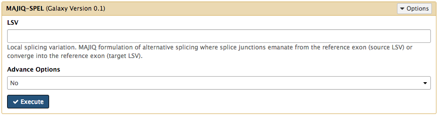
Paste the data copied from the LSV table in majiq into the LSV field.
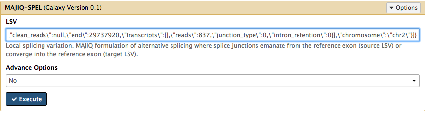
Click “Execute”. (Note that there are Advanced Options related to primer design that can be altered before submission described in detail here). Once the job has completed, click the “eye” icon next to the job to view MAJIQ-SPEL’s output. Now that the LSV has been digested by MAJIQ-SPEL, you’re now ready to begin designing primers.
MAJIQ-SPEL Primer Design
Now that we’ve completed the MAJIQ pipeline and were able to copy and paste an LSV into the MAJIQ-SPEL Galaxy Server submit form, we find ourselves with the MAJIQ-SPEL output. There are four sections to this page: Splice Graphs, General LSV Information, Primer Selection, and Isoform/PSI Plot comparison. Next, we’ll go over each section and describe their features.
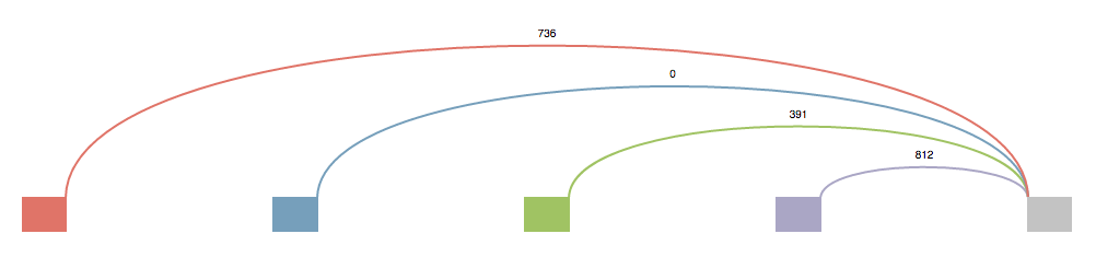
Splice Graphs
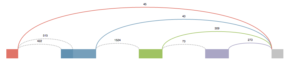
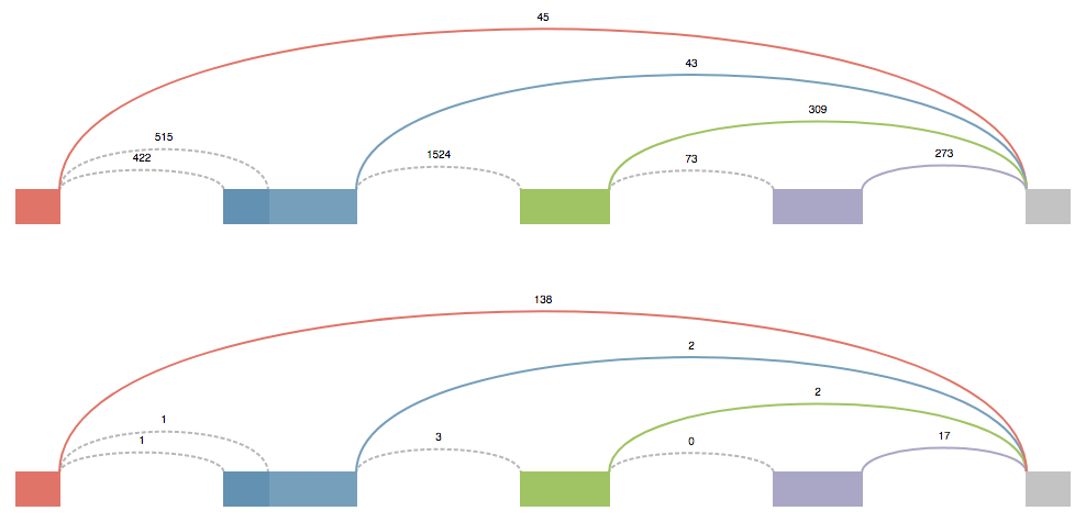
These splice graphs are highly modified version of the ones viewed in MAJIQ. They’re tailored to the needs of someone who is most concerned with designing primers. The splice graph doesn’t describe the entire gene, but instead it show’s the section of the gene where the LSV is located. It could be thought as an extended LSV. This modified splice graph has all the junctions, exons, and introns of an LSV, plus all the extra parts to travel from one side of the LSV to the other that contribute to the possible local isoform variations generated from the LSV.
Above each junction is the read counts. This value is directly pulled from the splice graph information found in MAJIQ and corresponds to the raw junction spanning read counts found in the bam files. (Note These raw read counts do not take into account a number of normalization factors that MAJIQ applies when quantifying an LSV like GC content correction, stack removal, read rate modeling, etc. For more details, see Vaquero-Garcia 2016).
Each junction that has been quantified will have a solid color. Any junction that has a dotted line (sometimes referred to as “No color”) is a junction that was not quantified directly in this LSV (and thus does not have an associated PSI Plot), but does contribute to the possible local isoform variations generated by the LSV.
The source/target reference exon for the LSV will always be gray. All other exons will either have a color or have a dotted outline. The dotted outline signifies that the junction from the gray exon to this exon isn’t quantified, but does play a role in an isoform for this LSV. Exons that have a color, obtain that color from the junction that is coming from the gray exon to it. Mousing over a junction will highlight that junction and bring it to the front.
General LSV Information
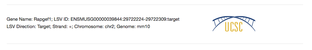
Below the splice graph is some general information about the LSV used to create this page. Such information as Gene ID, LSV ID, Genome, etc. can be used to help reference the LSV back to the Voila visualization or to the UCSC Genome Browser.
To view the LSV and the found forward and reverse primers within the UCSC Genome Browser, click the UCSC icon next the the general LSV information. In a section below, we’ll go over the LSV/Primer visualization within the Genome Browser.
Primer Selection
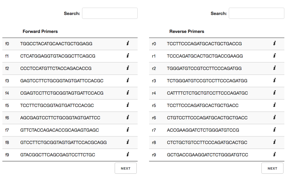
In the primer selection section of the page, there are two tables with three columns each. The first column is primer ID. This ID is generated specifically for this page and can be used to map this primer to the primer in the UCSC Genome Browser. Forward and reverse primer IDs start with an “f” and “r”, respectively.
The second column is the nucleotide string for the primer. These can be used in BLAT searches with the Genome Browser. Also, they can be used to search the primer tables for similar primers.
The last column is the “i” icon. When this icon is clicked a table of primer specific information will slide down. This additional primer information includes primer length, melting temperature, GC content, etc..
Primer Filters
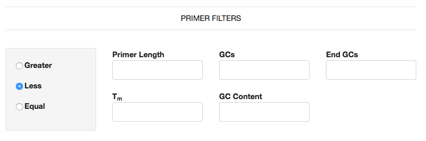
These filters allow you to further reduce the putative primers displayed in the tables on the fly, without having to re-execute SPEL. Additionally if you wish to further filter putative primers, you can utilize Primer3 (Untergasser et al., 2012, available at http://bioinfo.ut.ee/primer3/) where you can specify your specific RT-PCR assay conditions to rank and chose the optimal primer pair.
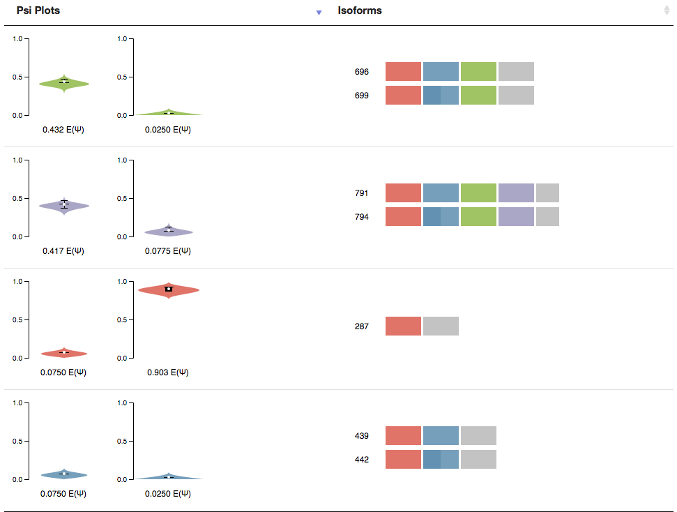
Isoform/PSI Plot Comparison
The final section of the page is a table containing the PSI Plots from MAJIQ and the local isoforms found by MAJIQ-SPEL. Next to each isoform is the nucleotide length of that isoform. This value will be recalculated when a two primers, that are found to be valid pairs, are selected.
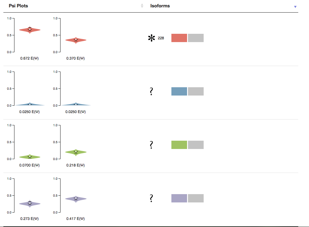
You will note two Icons that may appear next to the PCR product once a forward and reverse primer are selected. The “question mark” icon indicates that this isoform will not be amplified using the selected primers. Because the forward and reverse primers form MAJIQ-SPEL are specific to the 3’ and 5’ most exons in the LSV (red exon and grey exon in the above example), isoforms involving things like alternative transcription start sites (in the above example) or end sites will not be amplified. The other icon is the “asterisk” and it signifies that this isoform is particularly long, and thus may not be ideal for amplification via RT-PCR and may not resolve well on a gel. The Advance Option “Max Length” sets the limit for this flag.
The PSI Plots connects the MAJIQ PSI quantification for each condition to the relevant local isoform variations found by MAJIQ-SPEL. Note that because MAJIQ quantifies the relative usage of each junction (percent selected index or PSI), sometimes multiple local isoform variations are associated with a single PSI plot.
UCSC Genome Browser
To better understand how the primers are placed in comparison with the LSV and to facilitate downstream, functional analysis, we supply an annotation file that will be uploaded to the Genome Browser when UCSC icon is clicked. This file contains multiple custom tracks.
Exons and Junctions
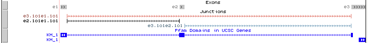
Exons and junctions are visualized in the Genome Browser as, shown in the above example. The color of the junctions will be the same as in MAJIQ-SPEL where junctions directly quantified by the LSV will be colored while those not directly quantified will be grey.
Pfam protein domains
The annotation file uploaded to the Genome Browser also contains annotated protein domains from Pfam (blue track in above example), which can aid users in downstream, functional analysis of local isoform variations.
For example, in the above case displays a de novo exon skipping in the RNA binding protein, Fubp3. The Pfam tracks indicate that exon 2 in this LSVs overlaps a large portion of the annotated KH RNA-binding domain, suggesting that this brain-specific exon skipping event would likely alter the RNA-binding ability of Fubp3.
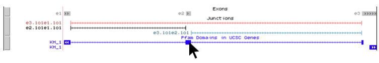
For additional information on the Pfam domain(s) that may overlap the your LSV of interest, simply click anywhere on the blue area(s) in the “Pfam Domains in UCSC Genes” track. In the example below we are interested in learning more information on the “KH_1” domain that overlaps our alternative exon.
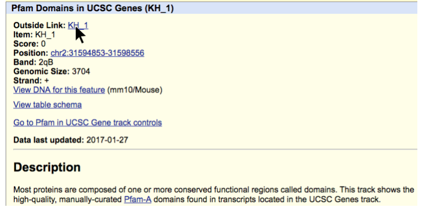
Clicking the blue track above brings up the Pfam Domains in UCSC Genes feature description page, shown below. By clicking on the “Outside Link” for “KH_1”, as shown below, we will be brought to the Pfam database page about this domain.
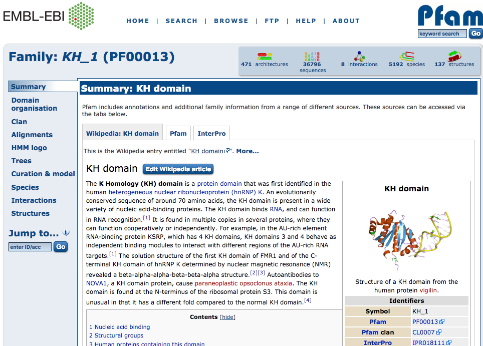
The Pfam database page for KH domain is shown below and we see this is an RNA binding domain. This page contains a wealth of additional information about the protein domain including what is know in the literature, structural information, sequence homology, interaction partners, etc. Using this information we can make predictions as to how an LSV that adds or removes peptide sequence to an annotated domain may alter the protein’s function.
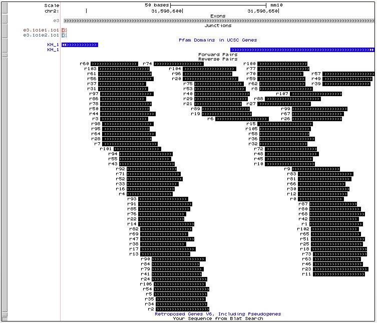
Forward and Reverse Primers
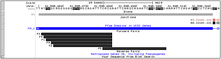
In the above image we see the found forward primers for our example LSV. This gives the location of the primers in relation the exon where a primer would begin where the IDs correspond to IDs in the primer table and could aid users in selecting their ideal primers for validation.
Galaxy Input Form - Advance Options
MAJIQ-SPEL is a Galaxy Server tool and like all Galaxy tools it will have a submit form. The submit form can be very simple much like the example in the previous section, or it can be expanded to reveal knobs to be tweaked. The drop down for Advanced Options defaults to “No”, but when “Yes” is selected many options will appear.
If you decide that you’d like to alter the Advance Options for a previous run, it would be easiest to click the “Run this job again” icon within Galaxy. To find this icon, click the name of the job you wish to run again in the right column and extra icons should appear below the job name. The “Run this job again” button looks like two arrows in a circle.
Each Advance Option is described below:
Min Length Exclude Limit
The minimum length of the smallest product amplified by forward and reverse primer pair. This prevents very small PCR products that would likely run off a gel.
Max Length
A flag will be displayed next to all isoforms that have a length longer than this value since large products are not amplified as well by RT and will not resolve well on a gel.
GCs Content Min/GCs Content Max
The minimum and maximum allowed GC content for each primer. GC content is calculated by the number of GCs / primer length.
Primer Length Min/Primer Length Max
The minimum and maximum length allowed for any primer.
Tm Min/Tm Max
The minimum and maximum melting temperature allowed for a primer based on the selected melting temperature formula.
GCs 3' Min/GCs 3' Max
The minimum and maximum number of GCs allowed at the 3’ end of the primer.
Melting Temp Formula
Select the melting temperature formula used to estimate the melting temperature of the primer. Currently there are two formulas to select from: Marmur and Wallace.
FAQ
When I download my MAJIQ-SPEL output from galaxy, it doesn't load in my browser?
The downloaded index.html from galaxy is viewable through a HTTP daemon. Otherwise, it will never load.
How do I install MAJIQ-SPEL on my local machine and run it?
MAJIQ-SPEL was build to run as a Galaxy tool. There are no guarantees that this will ever work reliably on the command line, but some work has been done to assist in debugging this software. See the software README for more information.
How many LSV juction colors are there?
MAJIQ-SPEL will use up to 11 colors. The number of LSVs that have more then 11 junctions are very rare. For example, Using the Hogenesch data ran through MAJIQ PSI we'll identify around 725,603 LSVs and we found about 140 of them to have 12 or more junctions. For this data set, 0.019% of LSVs will have more then 11 junctions.
For rare cases, where a user might have more then 11 junctions, MAJIQ-SPEL's color will wrap. This means the 12th colored junction will have the first color. Also, this means there will be a least two PSI plots with the same color. Even though different plots share the same color, the correct isoform will appear next to it.
References
Vaquero-Garcia, J., Barrera, A., Gazzara, M. R., Gonzalez-Vallinas, J., Lahens, N. F., Hogenesch, J. B., Lynch, K.W. & Barash, Y. (2016). A new view of transcriptome complexity and regulation through the lens of local splicing variations. Elife, 5, e11752.